

Having covered the fundamental things that make SpaceX able to take risks and create a milestone product in the first article, “The secret is in two details: how SpaceX engineers do the impossible“, here we will delve into the detailed technical analysis that guides Starship’s progress. We will start by breaking down how Mach contours affect aerodynamic design, and then look at the moving body simulations that capture Starship’s dynamic behavior. Finally, comments from the development team will provide insight into how this analysis is turned into real engineering decisions.
How SpaceX managed to design grid fins and interstage vents in ultra-short time and what it took to do it
By combining Mach Contours* analysis to predict aerodynamic effects at high speed with Integrated Flight Test 2 (IFT-2) flight data to validate and refine these predictions, SpaceX ensures that grid fins have the necessary control effects at various speeds and interstage vent safely manages pressure without compromising flight stability. This approach allows the behavior of the systems to be simulated as accurately as possible, even under the most challenging real-world flight conditions. It also helps minimize risks and ensures the rocket system’s high reliability during key mission phases.
Please read the article at the link to learn about the concept of the approach to analysis and engineering on an interstage vent of rocket carriers.
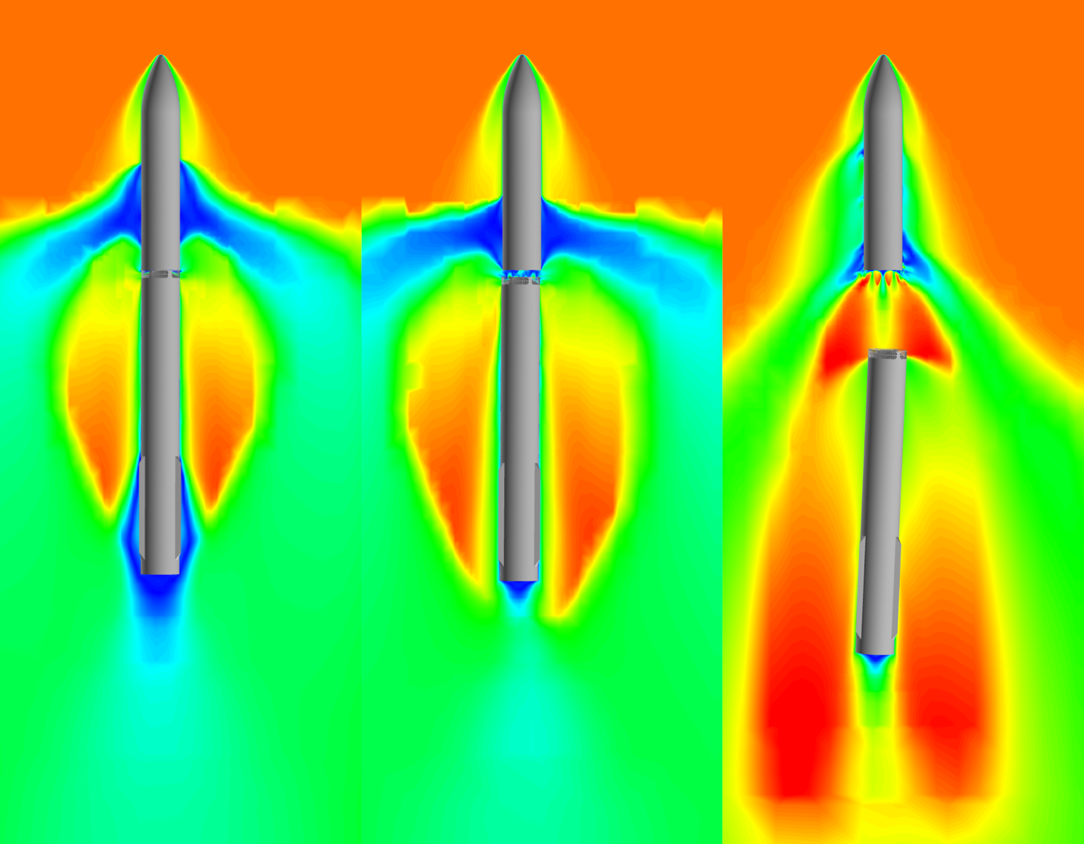
Each image uses a color scale (from cooler blue to warmer orange) to highlight the flow characteristics around the apparatus. In the first image, the upper stage booster and upper stage remain attached, with a relatively uniform flow around the body. The middle image shows the beginning of separation as the upper stage engine ignites while it is still attached to the booster, causing distinct aerodynamic effects and a prominent transition area between the stages. In the third image, the stages are completely separated; a pronounced high-temperature flow (orange area) can be seen around the ignited upper stage and a separate flow field surrounding the booster. The color gradients illustrate how the separation of the hot stages changes the pressure and velocity distributions in real time, giving engineers insight into critical locations influenced by complex aerodynamics.
*Mach Contours are a visual representation of the Mach number distribution in the flow field. Mach number is the ratio of the speed of flow to the speed of sound in that medium. During engine startup, especially for jet engines, turbomachines, or rocket engines, Mach contours are used to show how the flow field changes as the engine transitions from resting to operating conditions. This visualization helps engineers understand how air or exhaust gases behave in the engine and its environment during this critical period.
STEP I. Analysis of Mach number contour and grid fins at Raptor engine startup
The analysis yields design parameters in operating modes in the context of high-speed aerodynamics, specifically:
Shock wave location: the Mach contours show where supersonic shock waves form on the object, which is critical for grid design.
Pressure and heat load: At high Mach numbers, local pressure surges and heat transfer can increase dramatically around protruding structures (e.g. grid ribs and vents). Mach contour analysis accurately identifies these areas, controlling the choice of materials and structural reinforcement.
Vent flow interaction: interstage vent must safely vent gases without causing harmful flow disturbances. Mach loop studies show how the supersonic airflow interacts with the vented gases, preventing potential impact-induced damage or unstable flight behavior.
For this class of problems, the computational meshes consist of 500+ million elements. This grid size is roughly twice the size of the Space Launch System (SLS) launch environment simulation. It took months and even years to complete. To help SpaceX’s pre-launch design team, this modeling had to be completed in one week.

This animation is a representation of the Mach contour distribution during engine ignition and shows how it affects the surrounding airflow and helps validate the Starship’s design for supersonic operation.
SpaceX engineers faced a computational hurdle related to Starship’s complex grid geometry. The thin walls of each rib, large surface area, and fine details added more than 50 million grid elements to the simulation – so many that combining the entire model exceeded current computational limitations. This forced the team to be creative in modeling and analyzing these critical control surfaces, ensuring that Starship’s design remained within an acceptable range of deviation from the planned aerodynamic performance.
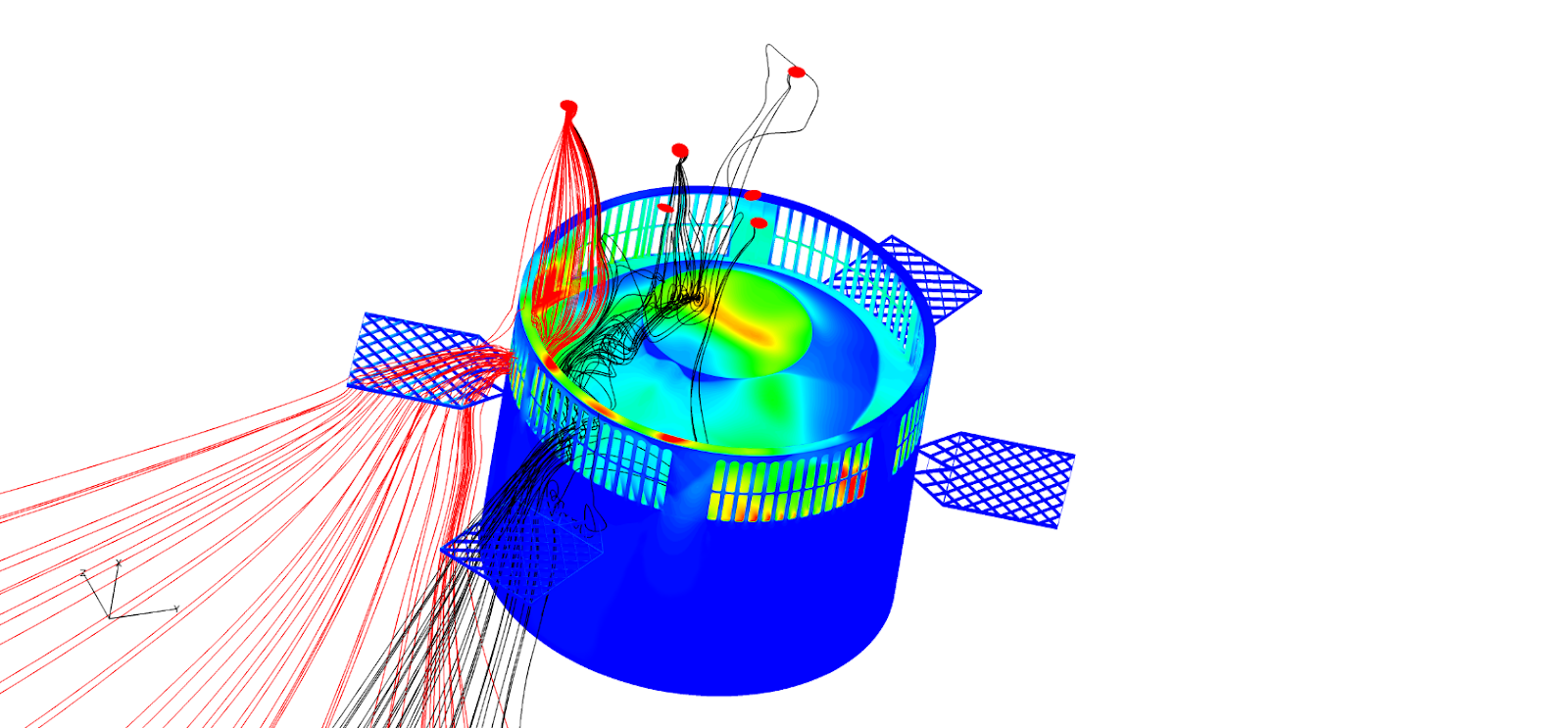
The main cylindrical structure (blue) represents an interstage section with four fins. A colored map on the surface indicates a flow-related variable – often a pressure or velocity value – where warm colors (yellow/orange) indicate higher values and cool colors (blue) indicate lower values. The black and red colored lines departing from specific points are streamlined lines illustrating how the fluid moves.
Patents and materials covering the design and calculation of grid fins often discuss aerodynamic optimization. In practice, CFD analysis is a key tool for modeling supersonic and subsonic flows around these complex grid structures, verifying the effectiveness of the fins for vehicle control. One such example is freely available at the link. For subscribers of the scientific publication Physics of Fluids, we recommend to read the material on the approach to grid fins calculations.
*CFD (Computational Fluid Dynamics) analysis is the use of computer simulation to model fluid flow around or within physical objects or systems. By applying mathematical equations and numerical algorithms, engineers can predict how factors such as pressure, temperature, and velocity will behave under different conditions. This provides detailed insights into aerodynamics, thermal performance or even chemical mixing, helping to improve designs and minimize the need for costly physical testing.
How can a team manage to calculate that in such a short time?
To solve such an ultra-complex problem in the context of timing, accuracy and reliability, the engineering team must perform a large amount of training to adapt the problem to simplify it. In the calculation of such a system, the main load parameter for the system that will compute the task is the number of grid elements and the design conditions that will act on each element. So what did the SpaceX team have to go through to accomplish this task?
- Mesh adaptation (mesh*)
The analysis of critical areas based on the results of previous calculations allowed us to adapt the total number of elements by increasing the mesh element size in non-critical areas concerning constant loads.
Provide high density in critical areas such as boundary layers, areas with high gradients or with complex initial flow conditions. Using adaptive mesh or using the “body of influence geometry” (BOI) within the working body based on the desired parameters.
Integration of tools for automatic mesh refinement as “adaptive mesh refinement” (AMR) in CFD solvers, which allowed automatic mesh refinement in critical areas.
AMR is a very convenient adaptation method that can save a lot of time for engineers, especially in simple or approximate calculations. A useful collection of articles on the use of this tool in various tasks can be found on Sciencedirect.
*In simple words, a mesh is like a digital network or mesh that breaks a 3D object or space into small, simple shapes (such as cubes, triangles, or other polygons). These shapes are called elements, and they help calculate air, water, or heat, movement, or behavior around or within the object.
- Reducing complexity in geometry
In the preliminary design phase, engineering design work and applied calculation activities run almost in parallel. Therefore, simplification of small elements or complex parts of the geometry that do not significantly affect the flow is a basic necessity to simplify calculations. A favorable condition for accepting tradeoffs between design, manufacturability, and geometry for calculations that need to be agreed upon in short time frames and risk acceptance is the appropriately constructed decision-making structure at SpaceX.
- The use of symmetry
For certain computational cases where the model and flow conditions are symmetric, only a portion of the geometry (e.g., half or quarter) is simulated and symmetry boundary conditions are applied to significantly reduce the computational volume.
- The initial parameters and solution methods are perfectly specified
The correct turbulence model is chosen and the boundary layer density is balanced.
The geometry of the mesh elements is specified according to key areas, for example, polyhedral meshes provide accuracy with fewer elements and tetrahedral meshes provide high quality for complex geometries.
High performance computing (HPC) or cloud computing clusters have been used.
- Simplification of physical and mechanical parameters
Utilizing k-epsilon flow physics instead of more computationally intensive models such as SST or LES. Analyze and understand areas where additional heat transfer calculations and multiphase physics can be omitted for simplification.
- Configuring simulation parameters
Carefully reduced simulation time and calculation time step size. Large time steps are used for steady-state or transient analysis, preserving stability and convergence acceleration techniques.
STEP II. IFT-2: Transient analysis of a moving body
Analyzing and validating the design in a real IFT-2 flight was necessary for the following reasons:
Full-scale conditions: Integrated Flight Test 2 provides real-world conditions – high Mach modes, dynamic pressure peaks, and cases of rapid stage detachment. These data points are important to verify that the grid ribs and interstage vents are operating as predicted by the simulation.
Transient analysis of a moving body: During IFT-2, the Starship’s orientation, thrust and aerodynamic load change rapidly. The grid ribs must react quickly to maintain control, and the interstage vent must cope with the changing pressure differential. Flight test measurements confirm whether the design can handle these transitions.
Model refinement and iterations: Post-flight analysis either confirms design assumptions or highlights areas for improvement. Engineers feed actual flight performance data back into computational models, updating Mach contour predictions and optimizing vents and grids configurations.
The experiment yielded the data shown in the diagram:
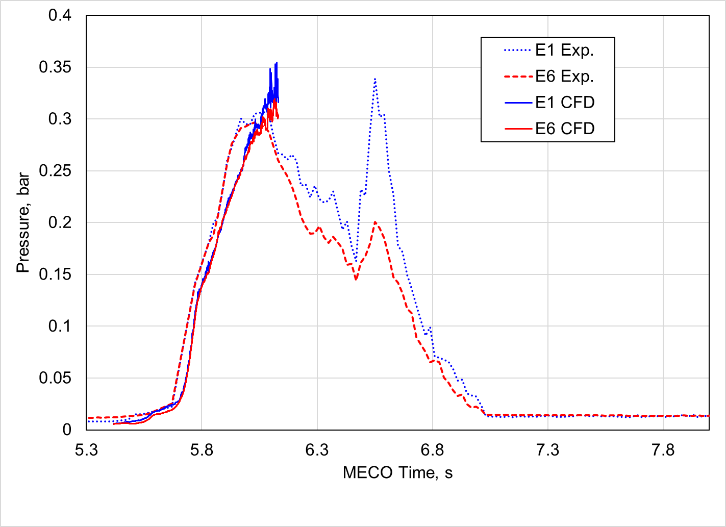
This diagram plots pressure (in bars) on the Y-axis against time (in seconds) on the X-axis, with a time window labeled around the Main Engine Cut-Off (MECO) process (approximately 5.3 s to 7.8 s). Four separate curves are displayed:
E1 Experimental (E1 Exp.) – shown with a blue dashed line
E6 Experimental (E6 Exp.) – shown with a dashed red line
E1 CFD – shown with a solid blue line
E6 CFD – shown with a solid red line
The diagram analysis provides engineers with a comparison between experimental (Exp.) and computational fluid dynamics (CFD) data, showing agreement in both the low-pressure rise and peak-pressure phases. Curves E1 (blue) show a particularly close agreement between the experimental and CFD predictions around the peak pressure region, indicating that the numerical model accurately captures the main flow characteristics. Meanwhile, the E6 curves (red) show a similar trend but exhibit more prominent deviations during the middle phase of the decline, indicating some local flow phenomena or boundary conditions that may not be fully captured by the modeling but should be accounted for in the next modeling iteration. However, the overall direction and similar dynamics emphasize the value of CFD as a predictive tool, and the importance of continuous improvement to increase accuracy in the rapidly changing transient conditions near the Main Engine Cut-Off (MECO) zone.
What do the participants themselves say about the process? How to plan the settlement process to get a successful result within the set deadline?
Jason Liu, MSFC-ER42 Fluid Dynamics Branch, a member of the Amentum Space Exploration Group:
“Plan ahead. As the first test flight with FITH approached, we anticipated the need for significant computational resources to complete the analysis. We worked with NASA HPC to reserve the necessary resources to meet our deadlines.
Be flexible. When critical times came with tight deadlines, we had three people who could devote all their time to completing and analyzing the right simulations.
Know the limitations of your tools. The size of these simulations is the limit of our software and NASA High Performance Computing (HPC). Judicious use of our tools has avoided mishaps (e.g., software failures) that could have delayed our deadlines.”
NASA’s Technical Reports Server has the primary source available.
Fail fast, learn faster
SpaceX’s “fail fast, learn faster” philosophy not only accelerates testing but also encourages rapid iterations in computational modeling. By applying fast results in both experimentation and analysis, engineers can adapt simulation parameters more creatively and efficiently – an approach that relies heavily on hands-on experience. Iterations between computation, analysis, and flight testing form the backbone of this development cycle.
Each new process insight gained from simulation and testing is quickly fed back into the model, improving it. This iterative cycle is vital to building reliable high-performance systems, emphasizing how thoughtful risk-taking and continuous learning are essential components of SpaceX’s current and future success.
